今回はPythonを使って日本株のデータを取得、グラフ表示をする簡単なプログラムを紹介します。
投資についてはずぶの素人で色々な本を読んでいると、「こういう形のチャートを探して…」という風な話が多いという印象を受けました。
とはいえ会社はたくさんあるので、一つ一つチャートを見ていくのは大変です。
ここら辺をPythonプログラムを使って効率化できたらいいのでは、と思い色々と調べているという感じです。
データの取得について
いくつか選択肢はあるみたいですが、investpyライブラリを使うのがよさそうです。
https://investpy.readthedocs.io/_info/introduction.html
冒頭分を引用します。
investpy is a Python package to retrieve data from Investing.com, which provides data retrieval from up to 39952 stocks, 82221 funds, 11403 ETFs, 2029 currency crosses, 7797 indices, 688 bonds, 66 commodities, 250 certificates, and 4697 cryptocurrencies.
investpy allows the user to download both recent and historical data from all the financial products indexed at Investing.com. It includes data from all over the world, from countries such as United States, France, India, Spain, Russia, or Germany, amongst many others.
investpy seeks to be one of the most complete Python packages when it comes to financial data extraction to stop relying on public/private APIs since investpy is FREE and has NO LIMITATIONS. These are some of the features that currently lead investpy to be one of the most consistent packages when it comes to financial data retrieval.
英語に関してもずぶの素人の私ですが、とりあえず無料で制限なしということは理解できました。
まだ試してないですが、探索系のプログラムを組む際に、約に立ちそうですね。
つかいかた
さっそくinvestpyの使い方を見ていきましょう。
まずはpip installです。
pip install investpy
直近の株価
直近の株価を取得するには以下のようにします。
題材として任天堂(7974)を使います。
import investpy
import pandas as pd

# 直近のデータ
df = investpy.get_stock_recent_data(
    stock='7974',
    country='japan'
)

print(df)
>>>
               Open     High      Low    Close   Volume Currency
Date
2021-09-21  51840.0  53020.0  51830.0  52660.0   652400      JPY
2021-09-22  53120.0  53770.0  53000.0  53240.0   825800      JPY
2021-09-24  54000.0  54500.0  53620.0  53800.0   800700      JPY
2021-09-27  54280.0  54820.0  54110.0  54180.0   727700      JPY
2021-09-28  53820.0  53870.0  52660.0  53430.0   893300      JPY
....
2021-10-15  51460.0  51690.0  50900.0  51530.0   742500      JPY
2021-10-18  51520.0  51890.0  51030.0  51260.0   575100      JPY
2021-10-19  51620.0  52590.0  51620.0  52350.0   627300      JPY
2021-10-20  51430.0  51600.0  49770.0  50300.0  1364100      JPY
2021-10-21  49690.0  50650.0  49370.0  50060.0   776100      JPY
一カ月分が表示されるみたいです
期間を指定して取得
df = investpy.get_stock_historical_data(stock='7974',
                                        country='japan',
                                        from_date='01/01/2020',
                                        to_date='01/01/2021')
print(df)
>>>
               Open     High      Low    Close   Volume Currency
Date
2020-01-06  43010.0  43090.0  42510.0  42740.0  1154600      JPY
2020-01-07  43040.0  43500.0  42890.0  42940.0  1167600      JPY
2020-01-08  42500.0  42840.0  41610.0  42640.0  1484400      JPY
2020-01-09  43550.0  43600.0  43160.0  43380.0  1030800      JPY
2020-01-10  43220.0  43780.0  43140.0  43440.0   826300      JPY
...             ...      ...      ...      ...      ...      ...
2020-12-24  64870.0  64870.0  64010.0  64730.0   606100      JPY
2020-12-25  64750.0  65090.0  64330.0  64670.0   520000      JPY
2020-12-28  64920.0  66150.0  64670.0  65880.0  1189300      JPY
2020-12-29  66290.0  66630.0  65560.0  65860.0   898600      JPY
2020-12-30  65560.0  66580.0  65460.0  65830.0   784700      JPY
名称から検索
和名は対応していないみたいですが、会社名から検索したりもできます。
使いみちがあるかはよく分かりません。
search_result = investpy.search_quotes(text='nintendo', products=['stocks'],
                                       countries=['japan'], n_results=1)
print(search_result)
>>>
{"id_": 946265, "name": "Nintendo Co Ltd", "symbol": "7974", "country": "japan",
"tag": "/equities/nintendo-ltd", "pair_type": "stocks", "exchange": "Tokyo"}
検索結果から、直近データや時系列データを取得することができます。
search_result = investpy.search_quotes(text='nintendo', products=['stocks'],
                                       countries=['japan'], n_results=1)
recent_data = search_result.retrieve_recent_data()
historical_data = search_result.retrieve_historical_data(from_date='01/01/2019', to_date='01/01/2020')
その他詳細は公式ページにて
https://investpy.readthedocs.io/_info/usage.html
mplfinanceを使ってグラフ化する
株価のデータが取得できたので次はグラフ化していきましょう。
今回はmatplotlibベースのmplfinaceを使っていきます。
pip install mplfinance2021/4/1~2021/10/1を表示期間とします。
import mplfinance as mpf
import pandas as pd
import investpy

df = investpy.get_stock_historical_data(stock='7974',
                                        country='japan',
                                        from_date='01/04/2020',
                                        to_date='01/10/2021')
mpf.plot(df)
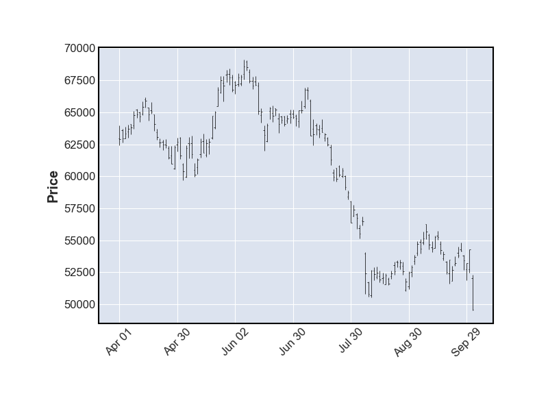
ちょっと見た目がやぼったいですね、引数を指定していくと、グラフをカスタマイズできます。
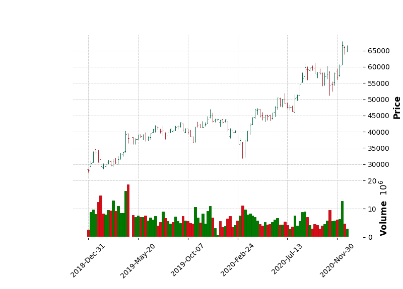
次は出来高を表示して、スタイルを当てる例です。
mpf.plot(df, volume=True, style='charles')
移動平均線を追加するには以下のようにします。
# 5日、25日、75日移動平均線の表示
mpf.plot(df, volume=True, style='yahoo', mav=(5, 25, 75))
週足、月足で見るときは元データを変換してグラフにします。
このあたりは地道に計算すると大変ですが、pandasが得意としている分野ですね。
以下のようにresampleメソッドを使うと簡単です。
df = investpy.get_stock_historical_data(stock='7974',
country='japan',
from_date='01/01/2019',
to_date='01/01/2021')
d_ohlcv = {'Open': 'first',
'High': 'max',
'Low': 'min',
'Close': 'last',
'Volume': 'sum'}
# 週足
df_w = df.resample('W-MON', closed='left', label='left').agg(d_ohlcv)
mpf.plot(df_w, style='charles', volume=True, )
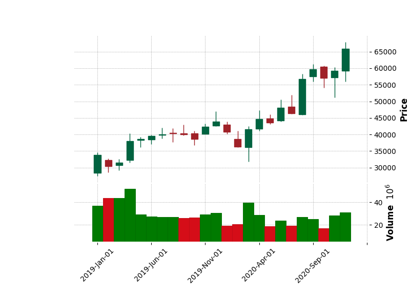
# 月足
df_m = df.resample('MS', closed='left', label='left').agg(d_ohlcv)
mpf.plot(df_m, style='charles', type='candle', volume=True, )
今回は2019年から2021年と少し期間を長くとってみました。
月足チャートはローソク足タイプに指定しています。
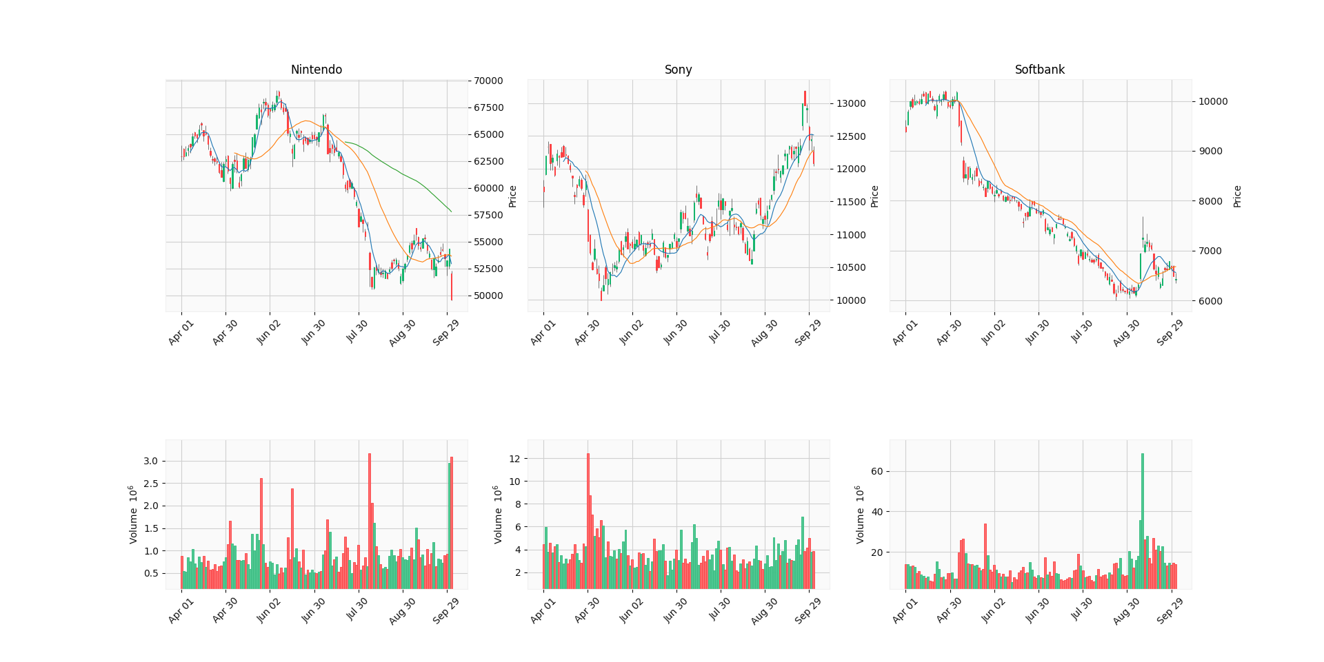
複数グラフをプロットする
複数のグラフを見比べる機会もあると思うので、使い方を確認しておきます。
matplotlibの複数グラフの作り方とおおむね同じです。
以下のようにします。
def get_historical_data(stock_code):
    return investpy.get_stock_historical_data(stock=stock_code,
                                              country='japan',
                                              from_date='01/04/2021',
                                              to_date='01/10/2021')

fig = mpf.figure(style='yahoo', figsize=(12, 8))
ax1 = fig.add_subplot(2, 3, 1)
ax2 = fig.add_subplot(2, 3, 2)
ax3 = fig.add_subplot(2, 3, 3)
av1 = fig.add_subplot(3, 3, 7, sharex=ax1)
av2 = fig.add_subplot(3, 3, 8, sharex=ax1)
av3 = fig.add_subplot(3, 3, 9, sharex=ax3)

nintendo = get_historical_data('7974')
sony = get_historical_data('6758')
softbank = get_historical_data('9984')

mpf.plot(nintendo, type='candle', ax=ax1, volume=av1, mav=(5, 25, 75), axtitle='Nintendo')
mpf.plot(sony, type='candle', ax=ax2, volume=av2, mav=(10, 20), axtitle='Sony')
mpf.plot(softbank, type='candle', ax=ax3, volume=av3, mav=(10, 20), axtitle='Softbank')

mpf.show()
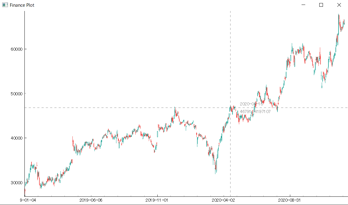
おまけ finplotを使う
matplotlibベースのmplfinanceを紹介してきましたが、finplotという良い感じのライブラリもあるみたいです。
pip install finplotimport finplot as fplt
import pandas as pd
import investpy
df = investpy.get_stock_historical_data(stock='7974',
country='japan',
from_date='01/01/2019',
to_date='01/01/2021')
fplt.candlestick_ochl(df[['Open', 'Close', 'High', 'Low']])
fplt.show()
カーソルを当てると詳細が確認できたりします。
githubページ
https://github.com/highfestiva/finplot
参考までに。
 Share
Share